The Tao of Trading - Adjusting the position

The Tao of Trading - adjusting the position - Ariel Faigon (2008)

Intro Case Pivot Position Simulation

The Optimal Position Size problem
Let's assume that we have already solved "the pivot problem". IOW: we already have a pivot at every point in time. We define the pivot as the "average asset price" relative to some time frame. In the optimal pivot article, we've already presented several techniques to calculate reasonably good pivots for different investor preferences and styles, from very active to rather passive.
Now trading becomes simple: buy when the price is below the pivot, and sell when it is above the pivot.
And the questions that remain are:

Whether the current price is far enough from the pivot to make the trade worthwhile.

How much to buy/sell

Of course, nothing is 100% guaranteed. Trading above and below the pivot is based on the reasonable expectation that more often than not the price will revert back to its mean, and that the mean is close enough to the pivot point. Even if sometimes it doesn't, the expectation is that whatever we do would be better than buying and holding, given enough time which will lead to trades. Also: since nothing is ever guaranteed, we should always diversify and have several generally non-correlated, assets on which we apply the method.
Many of you may be familiar with the "Secretary Problem":
en.wikipedia.org/wiki/Secretary_problem
These kinds of so called "stopping problems" are very relevant to investing. I'm looking for an optimal solution to a somewhat more complex problem but there's great similarity. In both cases we don't know the future, so we have to make a decision based on a (limited) past.
When faced with such problems, it is often useful to simplify if only for the sake of illustration, which makes it easier to gain insight.
Assume that we have only one asset. Like 'SPY' (the S&P500 index ETF) The asset moves up and down over time (this is a near 100% safe assumption for diversified and liquid assets). The base assumption is:
Short term movements in their aggregate are much larger than the net long-term trend. This is because over time most short term movements cancel each other (as we've convincingly seen here).

To optimize returns, we want to sell when the asset is relatively high, and buy when it is relatively low.
To make the solution more robust and realistic: we want to sell part of the asset when it is up, and buy somewhat more when it drops. Let our reference "zero point" be the smoothed line (recent N-day moving average of the asset). This isn't necessarily optimal, but as we've seen, a reasonable choice for a pivot line.
For the sake of illustration, let's assume that:

N is some constant, say 50-day.

The distribution of (past) moves around the N-day average is log-normal i.e. the daily change in percent is (approximately) normally distributed. This is key to avoiding a situation where we go broke by "doubling up" because the N-day moving average essentially follows the move of the asset. Eventually there must be some reversal to the mean where we lighten up.

We have limited funds. Practically, we can always stop the buying if we cannot add anymore, and we could also start with 50% position (compared to what we can afford overall) rather than with 100%, or we may assume that our broker lets us use 100% margin but no more. So our maximum position can be 200% (2.0) of our own capital, but never larger.

For the sake of simplicity, our 1st model assumes a neutral (sideways) market. See below for bull and bear modifications to the model.

The goal:
The goal is to maximize returns over-time using a single asset (the S&P 500 index) in a neutral market, by being active instead of buy-and-hold.
The problem:
What portion of the asset to sell (buy) when the asset is trading S standard-deviations above (below) the N-day smoothed line.

Here a shot at a reasonable modelling of the problem:
If 1.0 is our holding (whole portion), then our new position after every move (daily, weekly, whatever interval we chose to pick for our trading) should be:
P0 - L * 2 * (logistic(S) - 1.0))
Where logistic(S) is:
http://en.wikipedia.org/wiki/Logistic_function
And where P0 (position zero) is our position at the pivot. P0 is 1.0 for fully invested, 0.5 being half in cash, etc. L is our leverage, or the strength of our contrarian conviction. The greater L is, the bigger the position we feel comfortable taking against the short-term moves. Finally: S is the number of standard-deviations in which the asset trades above/below the pivot. S is determined using a sample of prices in some sliding window of time, typically one year (252 trading days).

The reason I chose this modified logistic function is that its value is y=0 where x=0, it never goes above 1 or below -1, when L=1.0, and lastly because it is monotonic and smooth. In short, it is well behaved and perfectly fulfills our need to increase/decrease the position against the asset short-term moves in a monotonic, smooth fashion.
Here's a chart of our modified logistic function, (assuming P0=0, L=1). Recall that we modify the classic logistic(x) by: a) multiplying by -2 and b) adding 1.0, in order to bring the Y-range to the interval [-1 .. 1])

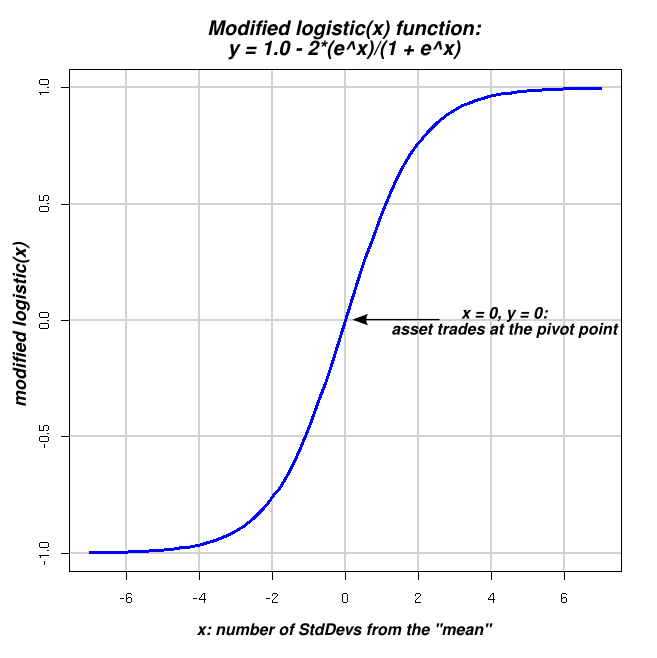
Note that the actual position we take is not the (modified) logistic. The logistic function should also be X-flipped around zero so our position moves contrary to the price. To achieve this, we can either negate x in the formula of the logistic function above, or negate the whole value (to flip around y=0). Both approaches have the same effect resulting in an inverted S shape which slopes down rather than up when moving from left to right.
Why L?
L is a nice constant to have
When L=0, and P0=1.0, the strategy becomes "buy and hold." The second term zeroes-out so you never change the initial 1.0 position. You're passive and always 100% invested.
As L grows, you become more aggressive/active as a trader; you trade against the movement, expecting the asset to revert to its mean baseline. It is essentially how much leverage you build into the system.
L = 1.0 is my current thinking of what 'optimal' reward/risk should be in a neutral (sideways) market.
When (L < 0) the activity means "pessimistically trading" i.e. "buying high and selling low," which is what most "emotional traders" do. Obviously it is a sure way to lose more and more money over time.
I also tried the 'double-logistic' function (see the bottom of the wikipedia article). Which has an additional (steepness) parameter. By choosing a good steepness parameter, we may be able to do a bit better with the double-logistic, I haven't explored this too deep yet because there's so much more low-hanging fruit to work on first.
Calculating the actual position percent as a function of S

Assuming P0=0 (100% cash at the pivot) and L=1, when the asset trades S standard deviations from the pivot, my new position in the two cases, becomes:
    logistic:		    - (2 * logistic(S) - 1.0)
    double logistic:	    - double_logistic(S, 0, 2.0)
Where S is the number of standard-deviations above/below the pivot line. Note that in contrast to buy-and-hold this strategy is 0% invested (all in cash) if the asset trades at the pivot (equilibrium point).
And to show some actual numbers, here are the positions at (+1.0 .. +3.0) stddev above and (-1.0 .. -3.0) stddev below the pivot line, all assuming (P0=0, L=1), negative percentages mean we're short:
Above (sell on spikes):

logistic:                 1.00 StdDevs from pivot    -46.21% invested
double-logistic(2):       1.00 StdDevs from pivot    -22.12% invested

logistic:                 2.00 StdDevs from pivot    -76.16% invested
double-logistic(2):       2.00 StdDevs from pivot    -63.21% invested

logistic:                 3.00 StdDevs from pivot    -90.51% invested
double-logistic(2):       3.00 StdDevs from pivot    -89.46% invested


Below line (buy on dips):

logistic:                 -1.00 StdDevs from pivot    46.21% invested
double-logistic(2):       -1.00 StdDevs from pivot    22.12% invested

logistic:                 -2.00 StdDevs from pivot    76.16% invested
double-logistic(2):       -2.00 StdDevs from pivot    63.21% invested

logistic:                 -3.00 StdDevs from pivot    90.51% invested
double-logistic(2):       -3.00 StdDevs from pivot    89.46% invested
As we can see the double-logistic function with the steepness=2.0 parameter is somewhat more conservative (keeps more in cash, and less invested except at the extremes), and thus may be somewhat more appropriate for periods of high uncertainty. We can also see that at the extremes (e.g. 3 StdDevs from the mean) the two functions tend to agree more as they asymptotically converge to 100% (or -100%) invested.
But... you say, "it is really dumb to be all in cash during bull markets," to which I fully agree which is the reason I designed the function assuming "neutral" market conditions. Most of the time, markets aren't neutral, and this is exactly what P0 (position at the pivot) is for. Let's look at P0 in more detail.

The P0 parameter: position at the pivot

P0 is another very useful constant to have
During bull markets (e.g. when the 100 day MA is above the 200 day MA of the index, or as long as leaders lead and the broader market confirms their higher highs), we set P0=1.0 in the position size formula. This means we are fully invested at the pivot point and get close to 100% cash, only if the asset trades well above the pivot. On the other extreme, we're getting leveraged (up to almost 200%) on the big dips. This setting is exactly what we want to have during bull markets when risks are low, and the tide tends to lift all boats. At these times, being less than 100% invested, is an inferior long-term strategy.
And during uncertain times when we're not sure, and the markets move mostly sideways, we can set P0=0 i.e. be 100% in cash when trading on the pivot, even better, during uncertain times we can lower our leverage to only about 50% (L=0.5), which will cause us to be only 50% invested at intermediate bottoms, and only about 50% "short" during spikes. To sum up:

Market type P0 Min position (spikes) Max position (dips)

Bull 1.0 0% 200%

Bear -0.5 -150% 50%
Neutral (uncertain) 0.0 -50% +50%

One last tweak to the position formula

Finally, I add one more (non-linear) optimization to reduce the chances of being caught on the wrong side of a large move: When shorting (on spikes) do it only for (1) assets which are long-term trending down. And when going long (on dips) do it only for (2) assets which are long-term trending up. We could determine trending either using the pivot line present direction (up or down) or slightly better: pick a longer time frame (e.g. 100-250 day SMA instead of 50 day SMA). During bear markets, we'll have more cases of type (1), and during bull markets, more cases of type (2). In fact, since we are allowed to use short ETFs, during bear markets, we would naturally be long those inverse ETFs, more often than the long ETFs.
Using inverse ETFs and applying the last two rules with appropriate values of P0 (midpoint position) and C (short term counter-movement leverage) makes our whole system more complete. Ultimately, we would have to figure out what strategy performs better on a risk adjusted basis, using back-testing.

The virtues of the logistic position formula

The logistic position formula with all the tweaks described above is, in my view, the ultimate investing discipline because it creates a rare blend of improved results while, at the same time, providing a strong psychological edge:

First, we just follow a cold formula. The process is 100% mechanical, and takes out the emotions from investing. Emotions invariably make results worse, controlling them is key to successful investing.

It frees us from having to worry about when (and how much) to sell. This is a major psychological edge. Whenever I sell "on a hunch", I'm left wondering if I have sold too early, or too late. With the logistic formula, there's no longer a single potential point of failure where one sells or buys. Rather, the position automatically, and gradually, changes to ensure a smoothed "buy relatively low" and "sell relatively high" on a continuous basis.

Our chances of "being right" increase: Since there's no way to know ahead of time whether the asset will peak 1.0 standard-deviations from the pivot, or 0.75, or whatever. Whatever happens, we do the "right thing", because we act on the past/present, not the future. If the asset moves down more, we buy more, if it moves less, we buy less, which is exactly the right thing to do given that the future is uncertain.

The continuous position adjusting, greatly smoothes-out the movements, thereby increasing our risk adjusted returns. This is because buying on dips and selling on spikes both reduces volatility, and realizes gains at the same time.

The contiuous position adjusting formula essentially says "let there be noise". We don't care how random the movements are as long as there's some reversion to the mean force. We don't argue with markets nor we try to anticipate long-term trands. The only thing we rely on is the undeniable existence of zig-zags in the price charts. We continuously, both adapt our pivot and harvest the stretching and reverting random-like movements around the pivot. We try to do this early and often.

Even if we were unlucky, and lost money overall, we've done better than buy and hold, because assets never go down in a straight line. With position adjusting, the more zigzags the asset makes -- which is exactly where 'normal' investors get nervous and fail -- the better we do.

The answer to life, the universe, and other things

With apologies to Douglas Adams: If you're a physicist, you should also love the analogy to the Fermi-Dirac distribution function:
F(x)=1/(1+exp(x))
Substitute x with -x, and you get the logistic function (to see why, divide both the nominator and the denominator of F(x) by exp(x)).
In Fermi statistics
F(x) = (E-Efermi)/kT
is the probability of a level with energy E to be occupied by a sub-atomic particle (for example by an electron).
Efermi is a parameter of the system, and kT is the Boltzman constant (k) times the temperature (T). Substituting x with -x is equivalent in this case to calculating 1-F(x), which is the probability the level is being unoccupied. I think the analogy to one of the most fundamental forces of nature is beautiful. Unoccupied to me means being a contrarian.

Intro Case Pivot Position Simulation

Disclaimer: this should not be considered as investment advice. It is merely describing my own thoughts and actions.
Feedback is welcome.
-- ariel